library(tidyverse)
library(tidymodels)
library(broom)

congress <- read_csv("data/congress.csv")Module 1 Lab: Election Forcasting
Introduction
U.S. Congressional House elections do more than just fill seats in government; they significantly impact the daily lives of people. Every ballot cast is a decision about which policies will shape the nation’s future, from healthcare and education to economic and environmental strategies. The elected representatives hold the power to craft laws that can affect job opportunities, healthcare access, and even the air we breathe. These elections, therefore, are not just a political ritual; they’re a crucial mechanism through which citizens exert direct influence on their own well-being and the direction of their community and country. Understanding this influence underscores the tangible consequences of each vote, reminding us that these democratic processes play a pivotal role in shaping the realities of everyday life.
At the same time, elections offer a revealing look into the psyche of American voters. For instance, Americans are increasingly polarized and entrenched in their political tribes. As behavioral scientists, elections offer a window into deep societal divides and group loyalties influence choices at the ballot box. In today’s politically charged environment, voters often align with their party’s broad brushstrokes, sometimes overlooking the finer details of a candidate’s policies or background. This trend highlights the strong role of group identity in shaping decisions. By examining the patterns and outcomes of these elections, we might better understand important psychological forces like thoes behind group loyalty and opposition.
Data
We will use data on U.S. House of Representatives Congressional Elections in 2014, 2016, 2018, and 2020. This data comes from the U.S. Federal Election Commission (fec.gov).
Exercises
We’re going to start by predicting election results in 2018 from the results the prior election in 2016.
Before we can really begin that though, we need to do some … drum roll please …
[ ]
]
Exercise 1
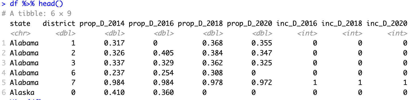
Our first step will be to set up our data so we can build our models. For each district, we will try to predict the share of votes won by the democratic House candidate. The first and most important predictor will be the democratic vote share from the prior election(s).
When you are done, a call of head() on your data should look something like this:
Warning
Make sure your df is not grouped to avoid unexpected behavior later as you split and add recipes.
Exercise 2
With our data ready in our df tibble, we can start building a model! Before we do that though, we need to split our data into training and testing splits. We might think more deeply about this in the future, but for now we can use the tidymodels default of 75% training 25% testing split.
Before splitting your data, set your random seed so that your results will match the answer key.
set.seed(1234)Exercise 3
Now we’ll start building our model specification and modeling workflow.
Exercise 4
Next we’ll fit the model (finally!).
Exercise 5
Check the fit of the model on the training data. We will focus on two ways of examining model fit. First, we’ll compute some metrics, including the Root Mean Squared Error and Mean Absolute Error (MAE). Second, we’ll plot the predicted values against the actual observed values.
Exercise 6
By looking at the predictions against the actual election results, we can see our model’s performance is somewhat mixed! Specifically, there are some elections that seem to be predicted quite well (the “cloud” of points along the 1:1 line), but others that are not (those kind of along the edges of the plot). What do you think is going on with the elections the model is failing to predict well?
Exercise 7
We’d like to add a predictor to our dataset to account for uncontested elections in our model. But, if we are going to add a new predictor we will need to also add it to our train and test splits. A better way to manage this kind of “feature engineering” is to use a recipe. The function step_mutate() can be used to engineer a new predictor in our dataset. By default, the created variable(s) are then automatically added as predictors to the model formula.
Let’s create a recipe and add that to the workflow.
TipWhat is a recipe?
A tidymodels recipe is a set of data manipulation and/or preprocessing steps carried out prior to fitting a model. A recipe can be combined with a model inside a workflow to take a set of data, preprocess it, and then pipe that through a model. Unlike calling mutate() on a dataframe, adding a call of step_mutate() in a recipe doesn’t modify the data right away. Instead, it just marks this as a step to complete when the recipe is called inside an appropriate workflow or function. In other frameworks the concept of a workflow is often called a “pipeline.” For more, see Lecture 4 of Module 1.
The Recipes package includes two helpful functions for previewing the results of a recipe. prep() and bake() can help you see what your recipe steps will accomplish, without having to train and fit a model. First you prep() the recipe, then you bake() the data using the prepped recipe.
The schema is:
the_recipe %>%
  prep() %>%
  bake(the_data)
Exercise 8
Now let’s examine the fit of our new model and compare it to the previous one.
Exercise 9
Now let’s try creating some new model specifications that use more predictors. We’ll add everything we legitimately can, so all predictors from 2016 or before as well as whether the election in 2018 is for an incumbent.
Tip
We can use a . in our formula to refer to all other variables. So if we set our formula to y ~ . we will tell the model to predict using all other variables. This is useful when we have a LOT of predictors in our model and we don’t want to type them all. It is also useful when we are using recipes to create new variables that don’t already exist in the original data.
If we don’t actually want to use all predictors, we can use the function step_select(..., skip = TRUE) to select only the subset we want (and to skip this step when predicting from an already-fit model).
Exercise 10
Exercise 11
Exercise 12
But wait, how would we actually use data or a model like this? The real usefulness of a model like this would be to predict the future.
Let’s take ourselves back to 2019—the federal government was shutting down, Felicity Huffman was in prison, “Old Town Road” was blaring everywhere, and an intrepid data scientist like yourself might be looking to forecast the likely results of the 2020 U.S. House election. Perhaps such a budding Nate Silver could use a model like the one we just created to do just that: using a forecasting model built from 2016 data to forecast by predicting 2020 vote shares from the 2018 data.
To reuse our model, we will cheat and rename our variables so that the model can generate predictions for 2020 using the 2018 data in place of the 2016 data and the 2016 data in place of the 2014 data.
Exercise 13
Wrapping up
When you are finished, knit your Quarto document to a PDF file.
When you are sure it looks good, submit it on Canvas in the appropriate assignment page.